
Batch Normalisation: From Scratch to Experiment
Published:
Batch Normalisation
Batch Normalisation was introduced in 2015, back when we were still struggling to train and converge deep neural networks (DNNs). Despite being almost 10 years old, it’s still a key technique used to stabilise and accelerate training.
The core problem BN tackles is internal covariate shift in hidden layers. Since network weights keep changing during training, the input distribution to later layers also shifts. This results in slower learning and can introduce saturation problems like exploding or vanishing gradients.
How Batch Norm Works
During Batch Norm, the activations are normalised for each feature (in each layer) across a mini-batch by calculating the mean and variance.
Given a batch $x = {x_1, x_2, …, x_m}$:
\[\hat{x}\_i = \frac{x\_i - \mu\_B}{\sqrt{\sigma\_B^2 + \epsilon}}\]where
- $\mu_B = \frac{1}{m} \sum_i^m x_i$ (batch mean)
- $\sigma_B^2 = \frac{1}{m} \sum_i^m (x_i - \mu_B)^2$ (batch variance)
A small $\epsilon$ is added for numerical stability.
Then we re-scale and shift the normalised activations using learnable parameters $\gamma$ and $\beta$:
\[y\_i = \gamma \hat{x}\_i + \beta\]This keeps the representation power of the layer intact, since normalisation alone might constrain the optimal distribution.
Implementing Batch Normalisation (From Scratch)
import torch
import torch.nn as nn

class MyBatchNorm1d(nn.Module):
    def __init__(self, num_features, eps=1e-5):
        super().__init__()
        self.gamma = nn.Parameter(torch.ones(num_features))
        self.beta = nn.Parameter(torch.zeros(num_features))
        self.eps = eps

    def forward(self, x):
        # x: (batch_size, num_features)
        mean = x.mean(dim=0, keepdim=True)
        var = x.var(dim=0, keepdim=True, unbiased=False)
        x_hat = (x - mean) / torch.sqrt(var + self.eps)
        return self.gamma * x_hat + self.beta

# Test implementation
x = torch.randn(8, 4)
bn = MyBatchNorm1d(4)
print(bn(x))
Example Output:
tensor([[-0.2802, -0.5166,  0.7289, -0.7232],
        [ 1.4447,  1.2645, -1.4518, -0.1239],
        [ 0.9441,  1.2976, -1.7226, -2.0962],
        [-0.9036,  0.1180,  0.4469,  0.1953],
        [-0.8302, -1.6203,  1.3921,  1.1150],
        [ 0.6040, -0.6471,  0.2150,  1.0123],
        [-1.6281, -0.7807,  0.4536,  0.8436],
        [ 0.6492,  0.8847, -0.0622, -0.2228]], grad_fn=<AddBackward0>)
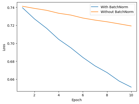
Experiment – With vs Without BN
Let’s compare training a simple MLP on the make_moons dataset with and without BatchNorm.
from sklearn.datasets import make_moons
import matplotlib.pyplot as plt
import torch
import torch.nn as nn
from torch.utils.data import TensorDataset, DataLoader

X, y = make_moons(n_samples=1000, noise=0.1, random_state=42)
X = torch.tensor(X, dtype=torch.float32)
y = torch.tensor(y, dtype=torch.long)

dataset = TensorDataset(X, y)
loader = DataLoader(dataset, batch_size=32, shuffle=True)

# Define models with and without BN

class MLP(nn.Module):
    def __init__(self, use_bn=False):
        super().__init__()
        layers = [nn.Linear(2, 64)]
        if use_bn:
            layers.append(nn.BatchNorm1d(64))
        layers.append(nn.ReLU())
        layers.append(nn.Linear(64, 2))
        self.net = nn.Sequential(*layers)

    def forward(self, x):
        return self.net(x)

model_no_BN = MLP()
model_BN = MLP(use_bn=True)

optim_no_BN = torch.optim.SGD(model_no_BN.parameters(), lr=1e-4)
optim_BN = torch.optim.SGD(model_BN.parameters(), lr=1e-4)

criterion = torch.nn.CrossEntropyLoss()

num_epochs = 10
epoch_loss_BN, epoch_loss_no_BN = [], []

# training loop
for epoch in range(num_epochs):
    running_loss_BN, running_loss_no_BN = [], []
    for Xb, yb in loader:
        out_BN = model_BN(Xb)
        out_no_BN = model_no_BN(Xb)

        loss_BN = criterion(out_BN, yb)
        loss_no_BN = criterion(out_no_BN, yb)

        optim_BN.zero_grad(); loss_BN.backward(); optim_BN.step()
        optim_no_BN.zero_grad(); loss_no_BN.backward(); optim_no_BN.step()

        running_loss_BN.append(loss_BN.item())
        running_loss_no_BN.append(loss_no_BN.item())

    epoch_loss_BN.append(sum(running_loss_BN)/len(running_loss_BN))
    epoch_loss_no_BN.append(sum(running_loss_no_BN)/len(running_loss_no_BN))
    print(f"Epoch {epoch}: BN Loss={epoch_loss_BN[-1]:.4f}, No BN Loss={epoch_loss_no_BN[-1]:.4f}")
Sample Output:
Epoch 0: BN Loss=0.7396, No BN Loss=0.7412
Epoch 1: BN Loss=0.7271, No BN Loss=0.7388
Epoch 2: BN Loss=0.7167, No BN Loss=0.7366
...
Epoch 9: BN Loss=0.6512, No BN Loss=0.7192
And the loss curves
plt.plot(range(1, num_epochs+1), epoch_loss_BN, label='With BatchNorm')
plt.plot(range(1, num_epochs+1), epoch_loss_no_BN, label='Without BatchNorm')
plt.xlabel('Epoch')
plt.ylabel('Loss')
plt.legend()
plt.show()
Wrapping Up
That’s it — a quick essentials-guide to Batch Normalisation. We saw:
- Why BN is useful (stability + faster convergence)
- How it works mathematically
- A from-scratch PyTorch implementation
- An experiment showing its effect
- Still one of the most practical tricks in the deep learning toolkit 🚀